Fibonacci soup

There’s a meme floating around on places such as /r/ProgrammerHumor and /r/mathmemes:

But what properties (mathematically) would such a soup have after many days? Specifically, if we start with two distinct soups and every day produce a new one that is a mix of soups from the previous two days, what kind of soup will we ultimately end up with? Turns out the solution is a neat application of first-year university maths so let’s dig in!

The recipe

Fibonacci soup is very simple to make:¹

1. On day $0$ serve soup $0$ (e.g. spinach)
2. On day $1$ serve soup $1$ (e.g. pumpkin)
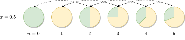
3. On day $n$ serve a soup consisting of a fixed proportion $x\in[0,1]$ of soup from $n-2$ days ago and a proportion $1-x$ of soup from the day before²

There is only one parameter $x$ which we could think of as “chef’s choice” which ultimately determines what kind of soup you get as $n$ grows large. Since on any given day a soup is a mixture of at most 2 initial soups (ingredients), we can focus on the evolution of the proportion of the first soup (served on day $0$)³. Denoting the proportion of the first soup on day $n$ by $p_n$ we have the following recurrence:

$$ \begin{aligned} p_0 &= 1 \\ p_1 &= 0 \\ p_n &= xp_{n-2}+(1-x)p_{n-1}. \end{aligned} $$

We can now work out a few simple cases “by hand” starting with the easy cases of $x=0$ and $x=1$. If $x=0$ then that means on day $n$ the soup is just the same as the one served on day $n-1$:

On the other hand if $x=1$, the soup on day $n$ is the same soup as served on day $n-2$:

Finally, let’s see what happens if $x=0.5$:

To find out how the proportions of the initial soups evolve for any $x$ we can either take the programmer’s approach or do some maths.

Programmer’s solution

We don’t have to think too much here—take the recurrence relation, write a function to iterate it and watch as results appear. In Python this might look something like this:

def soup(x = 0.5):
    p_0, p_1 = 1, 0
    while True:
      yield p_0
      p_0, p_1 = p_1, x * p_0 + (1-x) * p_1

N = 10
for n, p in zip(range(N), soup()):
    print(n, p)

0 1
1 0
2 0.5
3 0.25
4 0.375
5 0.3125
6 0.34375
7 0.328125
8 0.3359375
9 0.33203125

Looks like for $x=0.5$ the proportion of spinach soup is approaching $1/3$.

If we run this for a selection of values of $x$ we obtain the following plot:⁴

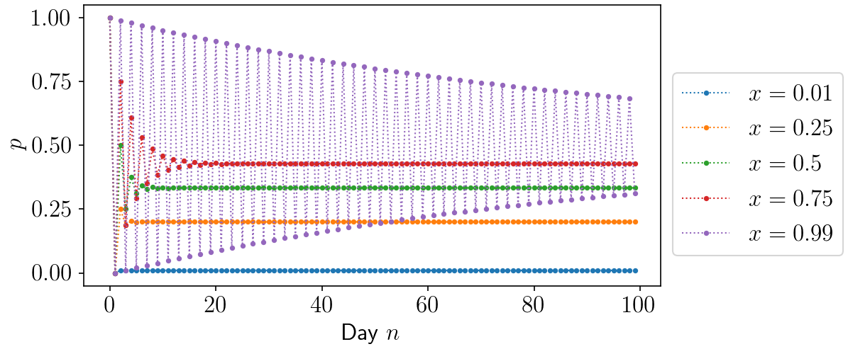
We notice several things:

• Lower $x$ results in much lower final proportion of soup $0$ (spinach)
• Any value of $x\in(0, 1)$ seems to converge to some final proportion of the initial soups
• Higher values of $x$ result in wild oscillations in the early days where on one day the majority ingredient might be spinach but on the following it would be pumpkin
• Higher values of $x$ take much longer to converge (for $x=0.99$ a hundred days are not enough) to a stable proportion, but they do seem to converge eventually

Nevertheless, to work out exactly what the final proportions of the initial soups are we need to turn to maths.

Mathematician’s solution

What we really want to know is the ultimate proportion of spinach to pumpkin soup as the number of days tends to infinity, in other words $\lim_{n\to\infty}p_n$. To do this we need to solve the recurrence relation. The recurrence is second order (since $p_n$ depends on the previous two terms of the sequence), linear (none of the terms appear as powers higher than one), homogeneous (there is no constant term), and has constant coefficients ($x$ and $1-x$ are independent of $n$). Given this we could look up a solution in a textbook or a wikipedia article.

The usual way these types of recurrences (also know as difference equations) are solved is similar to solving first and second order differential equations—we make an ansatz (a guess) of the form of the solution, work out the consequences and show that it is indeed a solution and then appeal to some uniqueness theorem to ensure that it is the only solution.⁵ In the case of our difference equation, we make an ansatz that the solution must be a power of the form $p^n$.⁶ Taking this ansatz and plugging it into the recurrence we get:

$$ p^n-(1-x)p^{n-1}-xp^{n-2}=0, $$ which must hold for all $n\geq 2$. Dividing through by $p^{n-2}$ we arrive at what is called the characteristic equation:

$$ p^2-(1-x)p-x=0. $$ This is a quadratic equation in $p$ with discriminant $(1-x)^2+4x=(x+1)^2$. Thus, the roots are:

$$ p_{\pm} = \frac{(1-x)\pm|x+1|}{2} $$ or $$ \begin{cases} p_{+} = 1 \\ p_{-} = -x. \end{cases} $$

The roots are both real, so the general solution will be:⁷ $$ \begin{aligned} p_n &= Ap_{+}^n + Bp_{-}^n \\ &= A + B(-x)^n, \end{aligned} $$ where the constants $A$ and $B$ are determined from the initial conditions $p_0$ and $p_1$. To find the constants, we plug in the values of $p_0=1$ and $p_1=0$ and solve the resulting system of equations:

$$ \begin{aligned} 1 &= A + B \\ 0 &= A - Bx. \end{aligned} $$ With some algebra we find: $$ \begin{aligned} A &= \frac{x}{x+1} \\ B &= \frac{1}{x+1}. \end{aligned} $$ Plugging these into the expression for $p_n$ and with some simplification we finally arrive at the solution:⁸ $$ p_n = \frac{1}{x+1}\left[x+\left(-x\right)^{n}\right], $$ which is valid for all $n\geq 0$ (try it yourself for $n=0,1,2$).

Now that we have a closed-form expression for $p_n$ we can analyse it’s convergence as a sequence. Fortunately it is quite easy in this case. If $x=0$, the whole expression reduces to $p_n=0$ which is what we had before.⁹ If $x=1$ the expression simplifies to: $$ p_n = \frac{1}{2}\left[1+(-1)^{n}\right]. $$ This gives us the oscillating behaviour between $1$ (spinach soup) and $0$ (pumpkin soup) we also observed before.

If $0<x<1$, we notice that due to the $(-x)^{n}$ term the expression in the brackets tends to $x$ as $n\to\infty$. Thus, $\lim_{n\to\infty}p_n=\frac{x}{x+1}$. In particular, for the case of equal mixing $x=0.5$ we get that eventually the ratio of spinach soup will be $\frac{1}{3}$ which is what we observed qualitatively in the pie charts and on the simulation results.

A final few observations:

• If $0<x<1$, the oscillations between consecutive days are due to $(-x)^n$ flipping between positive and negative values
• If $x$ is large, the oscillations at the start are bigger as $(-x)^n$ is bigger in absolute value but die down as $n$ grows
• If $x$ is large, the final proportions of the soup will be close to 50:50 (because $\lim_{x\to 1}\frac{x}{x+1}=\frac{1}{2}$).¹⁰

Epilogue

Even though Fibonacci soup is clearly a silly problem, surprisingly it packs enough interesting pieces to be, in my opinion, an interesting homework or exam problem for first year maths students. It touches on aspects of simulation, solving recurrences, analysing convergence of sequences, and still leaves room for further exploration (existence and uniqueness of the solution). Too bad we couldn’t taste any of the results!